Sam Foreman

Sam Foreman 2025-10-15

🌐 Distributed Training
🌌 AuroraGPT (2024–)
🧬 MProt-DPO
🌎 AERIS (2025)
📓 References
❤️ Acknowledgements

🌐 Distributed Training

🚀 Scaling: Overview

✅ Goal:
- Minimize: Cost (i.e. amount of time spent training)
- Maximize: Performance
[!NOTE]

📑 Note

See 🤗 Performance and Scalability for more details

In this talk, we will explore the intricacies of training foundation models on supercomputers. We will discuss the architecture of these models, the computational requirements, and the strategies employed to optimize training processes. Attendees will gain insights into the latest advancements in hardware and software that facilitate efficient model training at scale.

🐢 Training on a Single Device

flowchart LR
    subgraph G0["`GPU0`"]
        subgraph N0["`Network`"]
        end
        L0("`Loss`")
    end
    subgraph D["`Data`"]
        x("`x0`")
        x1("`x1`")
        x2("`x2`")
    end
    x --> N0
    N0 --> L0
    L0 --> N0
classDef block fill:#CCCCCC02,stroke:#838383,stroke-width:1px,color:#838383
classDef eblock fill:#CCCCCC02,stroke:#838383,stroke-width:0px,color:#838383
classDef red fill:#ff8181,stroke:#333,stroke-width:1px,color:#000
classDef green fill:#98E6A5,stroke:#333,stroke-width:1px,color:#000
classDef blue fill:#7DCAFF,stroke:#333,stroke-width:1px,color:#000
classDef grey fill:#cccccc,stroke:#333,stroke-width:1px,color:#000
class x,L0 red
class x1 green
class x2 blue
class x3 grey
class N0,G0,n0 block
class D eblock

Figure 1: SLOW !! model size limited by GPU memory

🕸️ Parallelism Strategies

Data Parallelism
- Split data across workers
- Easiest to implement
- No changes to model

Model Parallelism
- Split model across workers
Hybrid Parallelism
- Combine data + model parallelism
- More complex to implement
- Requires changes to model

👬 Training on Multiple GPUs: Data Parallelism

flowchart LR
    subgraph D["`Data`"]
        direction TB
        x2("`x2`")
        x1("`x1`")
        x("`x0`")
    end
    direction LR
    subgraph G0["`GPU0`"]
        direction LR
        subgraph N0["`NN`"]
        end
        %%y0("`y₀`")
        L0["`Loss`"]
    end
    subgraph G1["`GPU1`"]
        direction LR
        subgraph N1["`NN`"]
        end
        L1["`Loss`"]
    end
    subgraph G2["`GPU2`"]
        direction LR
        subgraph N2["`NN`"]
        end
        L2["`Loss`"]
    end
    x --> N0
    x1 --> N1
    x2 --> N2
    N0 --> L0
    N1 --> L1
    N2 --> L2
classDef block fill:#CCCCCC02,stroke:#838383,stroke-width:1px,color:#838383
classDef eblock fill:#CCCCCC02,stroke:#838383,stroke-width:0px,color:#838383
classDef text fill:#CCCCCC02,stroke:#838383,stroke-width:0px,color:#838383
classDef grey fill:#cccccc,stroke:#333,stroke-width:1px,color:#000
classDef red fill:#ff8181,stroke:#333,stroke-width:1px,color:#000
classDef orange fill:#FFC47F,stroke:#333,stroke-width:1px,color:#000
classDef yellow fill:#FFFF7F,stroke:#333,stroke-width:1px,color:#000
classDef green fill:#98E6A5,stroke:#333,stroke-width:1px,color:#000
classDef blue fill:#7DCAFF,stroke:#333,stroke-width:1px,color:#000
classDef purple fill:#FFCBE6,stroke:#333,stroke-width:1px,color:#000
classDef eblock fill:#CCCCCC02,stroke:#838383,stroke-width:0px,color:#838383
class x,y0,L0 red
class x1,L1 green
class x2,L2 blue
class x3,ar grey
class N0,N1,N2,G0,G1,G2,GU block
class D eblock
class AR block
class bc text

Figure 2: Each GPU receives unique data at each step

See 🤗 Methods and tools for efficient training on a single GPU

▶️ Data Parallel: Forward Pass

flowchart LR
    subgraph D["`Data`"]
        direction TB
        x("`x0`")
        x1("`x1`")
        x2("`x2`")
    end
    direction LR
    subgraph G0["`GPU0`"]
        direction LR
        subgraph N0["`NN`"]
        end
        L0["`Loss`"]
    end
    subgraph G1["`GPU1`"]
        direction LR
        subgraph N1["`NN`"]
        end
        L1["`Loss`"]
    end
    subgraph G2["`GPU2`"]
        direction LR
        subgraph N2["`NN`"]
        end
        L2["`Loss`"]
    end
    ar("`Avg. Grads (∑ₙgₙ)/N`")
    x --> G0
    x1 --> G1
    x2 --> G2
    N0 --> L0
    N1 --> L1
    N2 --> L2
    L0 -.-> ar
    L1 -.-> ar
    L2 -.-> ar
classDef eblock fill:#CCCCCC02,stroke:#838383,stroke-width:0px,color:#838383
classDef block fill:#CCCCCC02,stroke:#838383,stroke-width:1px,color:#838383
classDef grey fill:#cccccc,stroke:#333,stroke-width:1px,color:#000
classDef red fill:#ff8181,stroke:#333,stroke-width:1px,color:#000
classDef orange fill:#FFC47F,stroke:#333,stroke-width:1px,color:#000
classDef yellow fill:#FFFF7F,stroke:#333,stroke-width:1px,color:#000
classDef green fill:#98E6A5,stroke:#333,stroke-width:1px,color:#000
classDef blue fill:#7DCAFF,stroke:#333,stroke-width:1px,color:#000
classDef purple fill:#FFCBE6,stroke:#333,stroke-width:1px,color:#000
classDef text fill:#CCCCCC02,stroke:#838383,stroke-width:0px,color:#838383
class x,y0,L0 red
class x1,L1 green
class x2,L2 blue
class x3,ar grey
class N0,N1,N2,G0,G1,G2,GU block
class D eblock
class AR block
class bc text

Figure 3: Average gradients across all GPUs

◀️ Data Parallel: Backward Pass

flowchart RL
    subgraph D["`Data`"]
        direction TB
        x("`x0`")
        x1("`x1`")
        x2("`x1`")
    end
    subgraph G0["`GPU0`"]
        direction RL
        subgraph N0["`NN`"]
        end
        L0["`Loss`"]
    end
    subgraph G1["`GPU1`"]
        direction RL
        subgraph N1["`NN`"]
        end
        L1["`Loss`"]
    end
    subgraph G2["`GPU2`"]
        direction RL
        subgraph N2["`NN`"]
        end
        L2["`Loss`"]
    end
    subgraph BC["`Send Updates`"]
        direction TB
    end
    BC -.-> G0
    BC -.-> G1
    BC -.-> G2
    L0 ~~~ N0
    L1 ~~~ N1
    L2 ~~~ N2
    G0 ~~~ x
    G1 ~~~ x1
    G2 ~~~ x2
classDef grey fill:#cccccc,stroke:#333,stroke-width:1px,color:#000
classDef eblock fill:#CCCCCC02,stroke:#838383,stroke-width:0px,color:#838383
classDef block fill:#CCCCCC02,stroke:#838383,stroke-width:1px,color:#838383
classDef red fill:#ff8181,stroke:#333,stroke-width:1px,color:#000
classDef orange fill:#FFC47F,stroke:#333,stroke-width:1px,color:#000
classDef yellow fill:#FFFF7F,stroke:#333,stroke-width:1px,color:#000
classDef green fill:#98E6A5,stroke:#333,stroke-width:1px,color:#000
classDef blue fill:#7DCAFF,stroke:#333,stroke-width:1px,color:#000
classDef purple fill:#FFCBE6,stroke:#333,stroke-width:1px,color:#000
classDef text fill:#CCCCCC02,stroke:#838383,stroke-width:0px,color:#838383
class x,y0,L0 red
class x1,L1 green
class x2,L2 blue
class x3,ar grey
class N0,N1,N2,G0,G1,G2,GU block
class BC block
class bc text
class D eblock

Figure 4: Send global updates back to each GPU. See: PyTorch / Distributed Data Parallel

🔄 Collective Communication

Broadcast: Send data from one node to all other nodes
Reduce: Aggregate data from all nodes to one node
- AllReduce: Aggregate data from all nodes to all nodes
Gather: Collect data from all nodes to one node
- AllGather: Collect data from all nodes to all nodes
Scatter: Distribute data from one node to all other nodes

Reduce

Perform a reduction on data across ranks, send to individual

flowchart TD
  subgraph R0["`0`"]
    x0("`x0`")
  end
  subgraph R1["`1`"]
    x1("`x1`")
  end
  subgraph R2["`2`"]
    x2("`x2`")
  end
  subgraph R3["`3`"]
    x3("`x3`")
  end
  subgraph AR["`Reduce`"]
    xp["`z=reduce(x, 2, SUM)`"]
  end
  subgraph AR3["`3`"]
  end
  subgraph AR2["`2`"]
    xp2("`z`")
  end
  subgraph AR1["`1`"]
  end
  subgraph AR0["`0`"]
  end
  x0 --> AR
  x1 --> AR
  x2 --> AR
  x3 --> AR
  AR --> AR3
  AR --> xp2
  AR --> AR1
  AR --> AR0
classDef block fill:#CCCCCC02,stroke:#838383,stroke-width:1px,color:#838383
classDef red fill:#ff8181,stroke:#333,stroke-width:1px,color:#000
classDef orange fill:#FFC47F,stroke:#333,stroke-width:1px,color:#000
classDef green fill:#98E6A5,stroke:#333,stroke-width:1px,color:#000
classDef yellow fill:#FFFF7F,stroke:#333,stroke-width:1px,color:#000
classDef blue fill:#7DCAFF,stroke:#333,stroke-width:1px,color:#000
classDef purple fill:#FFCBE6,stroke:#333,stroke-width:1px,color:#000
classDef pink fill:#E599F7,stroke:#333,stroke-width:1px,color:#000
class R0,R1,R2,R3,AR,AR0,AR1,AR2,AR3 block
class xp,xp2 purple
class x0 red
class x1 green
class x2 blue
class x3 yellow

Figure 5: Reduce operation: one rank receives the reduction of input values across ranks

🐣 Getting Started: In Practice

📦 Distributed Training Frameworks:
- 🍋 saforem2 / ezpz
- 🤖 Megatron-LM
- 🤗 Accelerate
- 🔥 PyTorch
  - DDP / FSDP
🚀 DeepSpeed
- ZeRO Offloading
- Megatron-DeepSpeed

🧠 Memory Management:
- FSDP vs. ZeRO
- Activation Checkpointing
- Mixed Precision Training
- Gradient Accumulation
- Offloading to CPU/NVMe

[!IMPORTANT]

🔄 Keeping things in Sync

Computation stalls during communication !!

Keeping the communication to computation ratio small is important for effective scaling.

📝 Plan of Attack

flowchart TB
    A{"Model Perfect?"}
    A -- no --> M{"Available Memory?"}
    A -- yes --> AD["Done"]
    M -- yes --> MY["Make Model Larger"]
    M -- no --> ZMP["<b>Free Up Memory</b>"]
    MY --> A
    ZMP --> MY
    A:::block
    M:::block
    AD:::block
    MY:::block
    ZMP:::sblock
    classDef text fill:#CCCCCC02,stroke:#838383,stroke-width:0px,color:#838383
    classDef sblock fill:#CCCCCC02,stroke:#838383,stroke-width:1px,color:#838383,white-space:collapse
    classDef block fill:#CCCCCC02,stroke:#838383,stroke-width:1px,color:#838383

Figure 6: General strategy for scaling model training

🚀 Going Beyond Data Parallelism

✅ Useful when model fits on single GPU:
- ultimately limited by GPU memory
- model performance limited by size
⚠️ When model does not fit on a single GPU:
- Offloading (can only get you so far…):
  - DeepSpeed + ZeRO
  - 🔥 PyTorch + FSDP
- Otherwise, resort to model parallelism strategies

Going beyond Data Parallelism: DeepSpeed + `ZeRO`

Depending on the ZeRO stage (1, 2, 3), we can offload:
1. Stage 1: optimizer states $\left(P_{\mathrm{os}}\right)$
2. Stage 2: gradients + opt. states $\left(P_{\mathrm{os}+\mathrm{g}}\right)$
3. Stage 3: model params + grads + opt. states $\left(P_{\mathrm{os}+\mathrm{g}+\mathrm{p}}\right)$

Figure 7: DeepSpeed + ZeRO

🕸️ Additional Parallelism Strategies

Tensor (/ Model) Parallelism (TP):
- 🤗 Tensor Parallelism
- 🔥 Large Scale Transformer model training with Tensor Parallel (TP)
Pipeline Parallelism (PP):
- 🔥 PyTorch, DeepSpeed
Sequence Parallelism (SP):
argonne-lcf/Megatron-DeepSpeed
- Supports 4D Parallelism (DP + TP + PP + SP)

Pipeline Parallelism (PP)

Model is split up vertically (layer-level) across multiple GPUs
Each GPU:
- has a portion of the full model
- processes in parallel different stages of the pipeline (on a small chunk of the batch)
See:
- 🔥 PyTorch / Pipeline Parallelism
- DeepSpeed / Pipeline Parallelism

flowchart TB
    subgraph G0["`GPU 0`"]
        direction LR
        a0("`Layer 0`")
        b0("`Layer 1`")
    end
    subgraph G1["`GPU 1`"]
        direction LR
        a1("`Layer 2`")
        b1("`Layer 3`")
    end
    a0 -.-> b0
    b0 --> a1
    a1 -.-> b1
classDef block fill:#CCCCCC02,stroke:#838383,stroke-width:1px,color:#838383
classDef red fill:#ff8181,stroke:#333,stroke-width:1px,color:#000
classDef orange fill:#FFC47F,stroke:#333,stroke-width:1px,color:#000
classDef yellow fill:#FFFF7F,stroke:#333,stroke-width:1px,color:#000
classDef green fill:#98E6A5,stroke:#333,stroke-width:1px,color:#000
classDef blue fill:#7DCAFF,stroke:#333,stroke-width:1px,color:#000
classDef purple fill:#FFCBE6,stroke:#333,stroke-width:1px,color:#000
class G0,G1 block
class a0 red
class b0 green
class a1 blue
class b1 yellow

Figure 8: Pipeline Parallelism

Tensor Parallel (TP)

Split up network over multiple workers
Each receives disjoint subset
All communication associated with subsets are distributed
Communication whenever dataflow between two subsets
Typically more complicated to implement than data parallel training
Suitable when the model is too large to fit onto a single device (CPU / GPU)

Tensor (/ Model) Parallel Training: Example

Want to compute: $y = \sum_{i} x_{i} W_{i} = x_0 * W_0 + x_1 * W_1 + x_2 * W_2$
where each GPU has only its portion of the full weights as shown below

Compute: $y_{0} = x_{0} * W_{0}\rightarrow$ GPU1
Compute: $y_{1} = y_{0} + x_{1} * W_{1}\rightarrow$ GPU2
Compute: $y = y_{1} + x_{2} * W_{2} = \sum_{i} x_{i} W_{i}$ ✅

flowchart LR
    subgraph X0["`GPU0`"]
        direction LR
        a("`W0`")
    end
    subgraph X1["`GPU1`"]
        direction LR
        b("`W1`")
    end
    subgraph X2["`GPU2`"]
        direction LR
        c("`W2`")
    end
  t0("`x0`")-->X0
  X0 -->|"`x0 W0`"|X1
  X1 -->|"`x0 W0 + x1 W1`"|X2
  t1("`x1`") --> X1
  t2("`x1`") --> X2

Figure 11

🔭 AI-for-Science source (@tenderizzation)

ChatGPT: explain this image

$Forward Diffusion Process (\pi\rightarrow \mathcal{N})$

🌀 Sequence-Window-Pipeline Parallelism `SWiPe`

SWiPe is a novel parallelism strategy for Swin-based Transformers
Hybrid 3D Parallelism strategy, combining:
- Sequence parallelism (SP)
- Window parallelism (WP)
- Pipeline parallelism (PP)

Figure 23

Figure 24: SWiPe Communication Patterns

🚀 AERIS: Scaling Results

Figure 25: AERIS: Scaling Results

10 EFLOPs (sustained) @ 120,960 GPUs
See (Hatanpää et al. (2025)) for additional details
arXiv:2509.13523

🌪️ Hurricane Laura

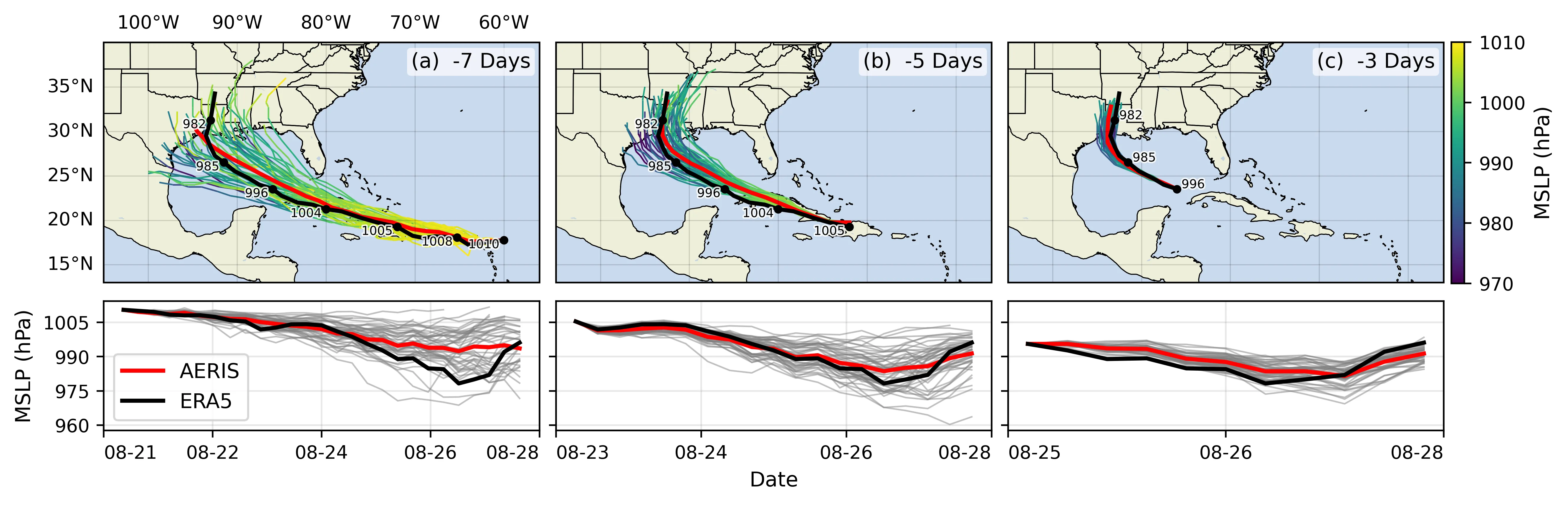
Figure 26: Hurricane Laura tracks (top) and intensity (bottom). Initialized 7(a), 5(b) and 3(c) days prior to 2020-08-28T00z.

📓 References

Hatanpää, Väinö, Eugene Ku, Jason Stock, et al. 2025. AERIS: Argonne Earth Systems Model for Reliable and Skillful Predictions. https://arxiv.org/abs/2509.13523.

Price, Ilan, Alvaro Sanchez-Gonzalez, Ferran Alet, et al. 2024. GenCast: Diffusion-Based Ensemble Forecasting for Medium-Range Weather. https://arxiv.org/abs/2312.15796.

Song, Shuaiwen Leon, Bonnie Kruft, Minjia Zhang, et al. 2023. DeepSpeed4Science Initiative: Enabling Large-Scale Scientific Discovery Through Sophisticated AI System Technologies. https://arxiv.org/abs/2310.04610.

❤️ Acknowledgements

This research used resources of the Argonne Leadership Computing Facility, which is a DOE Office of Science User Facility supported under Contract DE-AC02-06CH11357.

← <C-p> Previous

posts/ 06 Next <C-n> → talks/ AERIS: Argonne's Earth Systems Model

🌐 Distributed Training

🚀 Scaling: Overview

📑 Note

🐢 Training on a Single Device

🕸️ Parallelism Strategies

👬 Training on Multiple GPUs: Data Parallelism

▶️ Data Parallel: Forward Pass

◀️ Data Parallel: Backward Pass

🔄 Collective Communication

Reduce

🐣 Getting Started: In Practice

🔄 Keeping things in Sync

📝 Plan of Attack

🚀 Going Beyond Data Parallelism

Going beyond Data Parallelism: DeepSpeed + ZeRO

🕸️ Additional Parallelism Strategies

Pipeline Parallelism (PP)

Tensor Parallel (TP)

Tensor Parallel (TP)

Tensor (/ Model) Parallel Training: Example

🌀 Sequence-Window-Pipeline Parallelism SWiPe

🚀 AERIS: Scaling Results

🌪️ Hurricane Laura

📓 References

❤️ Acknowledgements

Going beyond Data Parallelism: DeepSpeed + `ZeRO`

🌀 Sequence-Window-Pipeline Parallelism `SWiPe`